Part I - Getting & wrangling data from the database
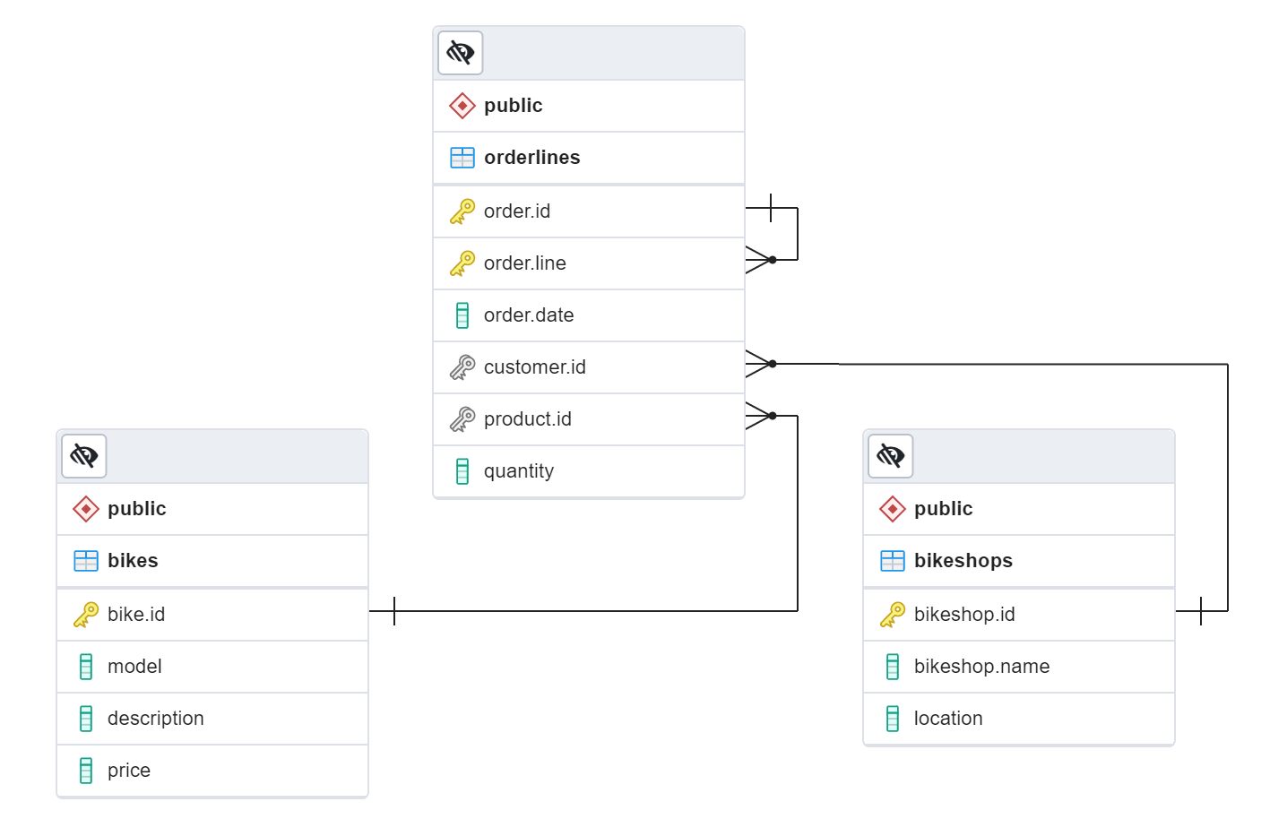
The Bike Sales Database represents a bicycle manufacturer, including tables for products (bikes), customers (bike shops), and transactions (orders).
It consists of 3 tables:
bikestable, which includes bicycle models, descriptions, and unit prices that are produced by the manufacturer.bikeshopstable, which includes customers that the bicycle manufacturer has sold to.orderlinestable, which includes transactional data such as order ID, order line, date, customer, product, and quantity sold.
bike_sales database is the local Postgres database stored on my machine.
Entity Relationship Diagram
Setting up the programming environment
# loading packages
library(DBI)
library(RPostgres)
library(tidyverse)
library(lubridate)
The sql engine uses the DBI package to execute SQL queries, print their results, and optionally assign the results to a data frame. To use the sql engine, we first need to establish a DBI connection to a database.
Creating a connection to the bike_sales database
mycon <- DBI::dbConnect(RPostgres::Postgres(),
                        dbname = "bike_sales",
                        host = "localhost",
                        port = "5432",
                        user = rstudioapi::askForPassword("Database username"),
                        password = rstudioapi::askForPassword("Database password"))
There are several options to secure your credentials in R. Here I use prompting for credentials via rstudioapi.
mycon<PqConnection> bike_sales@localhost:5432# list the database table names
dbListTables(mycon)[1] "bikeshops" "bikes" "orderlines"# read the bikeshops table
dbReadTable(mycon, "bikeshops") %>% head() bikeshop.id bikeshop.name location
1 1 Pittsburgh Mountain Machines Pittsburgh, PA
2 2 Ithaca Mountain Climbers Ithaca, NY
3 3 Columbus Race Equipment Columbus, OH
4 4 Detroit Cycles Detroit, MI
5 5 Cincinnati Speed Cincinnati, OH
6 6 Louisville Race Equipment Louisville, KY# read the bikes table
dbReadTable(mycon, "bikes") %>% head() bike.id model description price
1 1 Supersix Evo Black Inc. Road - Elite Road - Carbon 12790
2 2 Supersix Evo Hi-Mod Team Road - Elite Road - Carbon 10660
3 3 Supersix Evo Hi-Mod Dura Ace 1 Road - Elite Road - Carbon 7990
4 4 Supersix Evo Hi-Mod Dura Ace 2 Road - Elite Road - Carbon 5330
5 5 Supersix Evo Hi-Mod Utegra Road - Elite Road - Carbon 4260
6 6 Supersix Evo Red Road - Elite Road - Carbon 3940# read the orderlines table
dbReadTable(mycon, "orderlines") %>% head() order.id order.line order.date customer.id product.id quantity
1 1 1 2011-01-07 2 48 1
2 1 2 2011-01-07 2 52 1
3 2 1 2011-01-10 10 76 1
4 2 2 2011-01-10 10 52 1
5 3 1 2011-01-10 6 2 1
6 3 2 2011-01-10 6 50 1# a simple query example
dbGetQuery(mycon,
"SELECT model, price
FROM bikes WHERE price > 10000
ORDER BY price DESC") model price
1 Supersix Evo Black Inc. 12790
2 Scalpel-Si Black Inc. 12790
3 Habit Hi-Mod Black Inc. 12250
4 F-Si Black Inc. 11190
5 Supersix Evo Hi-Mod Team 10660Joining the tables
In all three tables there are dots in column names. This is not a good practice and I first had to figure out how to join the tables without an error! Here is the solution:
bike_orderlines_joined <- dbGetQuery(mycon,

'SELECT *
FROM orderlines
LEFT JOIN bikes
ON orderlines."product.id" = bikes."bike.id"
LEFT JOIN bikeshops
ON orderlines."customer.id" = bikeshops."bikeshop.id"')

head(bike_orderlines_joined)
order.id order.line order.date customer.id product.id quantity bike.id
1 1 1 2011-01-07 2 48 1 48
2 1 2 2011-01-07 2 52 1 52
3 2 1 2011-01-10 10 76 1 76
4 2 2 2011-01-10 10 52 1 52
5 3 1 2011-01-10 6 2 1 2
6 3 2 2011-01-10 6 50 1 50
model description price bikeshop.id
1 Jekyll Carbon 2 Mountain - Over Mountain - Carbon 6070 2
2 Trigger Carbon 2 Mountain - Over Mountain - Carbon 5970 2
3 Beast of the East 1 Mountain - Trail - Aluminum 2770 10
4 Trigger Carbon 2 Mountain - Over Mountain - Carbon 5970 10
5 Supersix Evo Hi-Mod Team Road - Elite Road - Carbon 10660 6
6 Jekyll Carbon 4 Mountain - Over Mountain - Carbon 3200 6
bikeshop.name location
1 Ithaca Mountain Climbers Ithaca, NY
2 Ithaca Mountain Climbers Ithaca, NY
3 Kansas City 29ers Kansas City, KS
4 Kansas City 29ers Kansas City, KS
5 Louisville Race Equipment Louisville, KY
6 Louisville Race Equipment Louisville, KYglimpse(bike_orderlines_joined)Rows: 15,644
Columns: 13
$ order.id <dbl> 1, 1, 2, 2, 3, 3, 3, 3, 3, 4, 5, 5, 5, 5, 6, 6, 6, 6, 7,…
$ order.line <dbl> 1, 2, 1, 2, 1, 2, 3, 4, 5, 1, 1, 2, 3, 4, 1, 2, 3, 4, 1,…
$ order.date <date> 2011-01-07, 2011-01-07, 2011-01-10, 2011-01-10, 2011-01…
$ customer.id <dbl> 2, 2, 10, 10, 6, 6, 6, 6, 6, 22, 8, 8, 8, 8, 16, 16, 16,…
$ product.id <dbl> 48, 52, 76, 52, 2, 50, 1, 4, 34, 26, 96, 66, 35, 72, 45,…
$ quantity <dbl> 1, 1, 1, 1, 1, 1, 1, 1, 1, 1, 1, 2, 1, 1, 1, 1, 1, 1, 1,…
$ bike.id <dbl> 48, 52, 76, 52, 2, 50, 1, 4, 34, 26, 96, 66, 35, 72, 45,…
$ model <chr> "Jekyll Carbon 2", "Trigger Carbon 2", "Beast of the Eas…
$ description <chr> "Mountain - Over Mountain - Carbon", "Mountain - Over Mo…
$ price <dbl> 6070, 5970, 2770, 5970, 10660, 3200, 12790, 5330, 1570, …
$ bikeshop.id <dbl> 2, 2, 10, 10, 6, 6, 6, 6, 6, 22, 8, 8, 8, 8, 16, 16, 16,…
$ bikeshop.name <chr> "Ithaca Mountain Climbers", "Ithaca Mountain Climbers", …
$ location <chr> "Ithaca, NY", "Ithaca, NY", "Kansas City, KS", "Kansas C…Disconnecting from the database.
dbDisconnect(mycon)Data wrangling
bike_orderlines <- bike_orderlines_joined %>%
  # rename columns - replacing "." with "_"
  set_names(names(.) %>% str_replace_all("\\.", "_")) %>%
  # remove the unnecessary columns
  select(-c(customer_id, product_id, bike_id, bikeshop_id)) %>%
  # separate description into category_1, category_2, and frame_material
  separate(description,
           c("category_1", "category_2", "frame_material"),
           sep = " - ") %>%
  # separate location into city and state
  separate(location,
           c("city", "state"),
           sep = ", ") %>%
  # create a new column total_price
  mutate(total_price = price * quantity) %>%
  # reorder columns
  select(contains(c("date", "id", "order")),
         quantity, price, total_price,
         everything())

bike_orderlines %>% head()
order_date order_id order_line quantity price total_price
1 2011-01-07 1 1 1 6070 6070
2 2011-01-07 1 2 1 5970 5970
3 2011-01-10 2 1 1 2770 2770
4 2011-01-10 2 2 1 5970 5970
5 2011-01-10 3 1 1 10660 10660
6 2011-01-10 3 2 1 3200 3200
model category_1 category_2 frame_material
1 Jekyll Carbon 2 Mountain Over Mountain Carbon
2 Trigger Carbon 2 Mountain Over Mountain Carbon
3 Beast of the East 1 Mountain Trail Aluminum
4 Trigger Carbon 2 Mountain Over Mountain Carbon
5 Supersix Evo Hi-Mod Team Road Elite Road Carbon
6 Jekyll Carbon 4 Mountain Over Mountain Carbon
bikeshop_name city state
1 Ithaca Mountain Climbers Ithaca NY
2 Ithaca Mountain Climbers Ithaca NY
3 Kansas City 29ers Kansas City KS
4 Kansas City 29ers Kansas City KS
5 Louisville Race Equipment Louisville KY
6 Louisville Race Equipment Louisville KYbike_orderlines %>% glimpse()Rows: 15,644
Columns: 13
$ order_date <date> 2011-01-07, 2011-01-07, 2011-01-10, 2011-01-10, 2011-0…
$ order_id <dbl> 1, 1, 2, 2, 3, 3, 3, 3, 3, 4, 5, 5, 5, 5, 6, 6, 6, 6, 7…
$ order_line <dbl> 1, 2, 1, 2, 1, 2, 3, 4, 5, 1, 1, 2, 3, 4, 1, 2, 3, 4, 1…
$ quantity <dbl> 1, 1, 1, 1, 1, 1, 1, 1, 1, 1, 1, 2, 1, 1, 1, 1, 1, 1, 1…
$ price <dbl> 6070, 5970, 2770, 5970, 10660, 3200, 12790, 5330, 1570,…
$ total_price <dbl> 6070, 5970, 2770, 5970, 10660, 3200, 12790, 5330, 1570,…
$ model <chr> "Jekyll Carbon 2", "Trigger Carbon 2", "Beast of the Ea…
$ category_1 <chr> "Mountain", "Mountain", "Mountain", "Mountain", "Road",…
$ category_2 <chr> "Over Mountain", "Over Mountain", "Trail", "Over Mounta…
$ frame_material <chr> "Carbon", "Carbon", "Aluminum", "Carbon", "Carbon", "Ca…
$ bikeshop_name <chr> "Ithaca Mountain Climbers", "Ithaca Mountain Climbers",…
$ city <chr> "Ithaca", "Ithaca", "Kansas City", "Kansas City", "Loui…
$ state <chr> "NY", "NY", "KS", "KS", "KY", "KY", "KY", "KY", "KY", "…Part II - Advanced plots with ggplot2
I will continue to work with the bike_orderlines dataframe and create two useful plots.
Lollipop Chart: Top N Customers
Question: How much purchasing power is in top 10 customers?
Goal is to visualize top N customers in terms of Revenue, including cumulative percentage.
Data manipulation
n <- 10

top_customers <- bike_orderlines %>%
  select(bikeshop_name, total_price) %>%
  mutate(bikeshop_name = as_factor(bikeshop_name) %>% fct_lump_n(n = n, w = total_price)) %>%
  group_by(bikeshop_name) %>%
  summarise(revenue = sum(total_price)) %>%
  ungroup() %>%
  mutate(bikeshop_name = bikeshop_name %>% fct_reorder(revenue)) %>%
  mutate(bikeshop_name = bikeshop_name %>% fct_relevel("Other", after = 0)) %>%
  arrange(desc(bikeshop_name)) %>%
  # revenue text
  mutate(revenue_text = scales::dollar(revenue, scale = 1e-06, suffix = "M")) %>%
  # cumulative percent
  mutate(cum_pct = cumsum(revenue) / sum(revenue)) %>%
  mutate(cum_pct_text = scales::percent(cum_pct)) %>%
  # rank
  mutate(rank = row_number()) %>%
  mutate(rank = ifelse(rank == max(rank), NA_integer_, rank)) %>%
  # label text
  mutate(label_text = str_glue("Rank: {rank}\nRev: {revenue_text}\nCumPct: {cum_pct_text}"))

top_customers
# A tibble: 11 × 7
bikeshop_name revenue revenue…¹ cum_pct cum_p…² rank label…³
<fct> <dbl> <chr> <dbl> <chr> <int> <glue>
1 Kansas City 29ers 11535455 $11.54M 0.162 16.2% 1 Rank: …
2 Denver Bike Shop 7697670 $7.70M 0.271 27.1% 2 Rank: …
3 Ithaca Mountain Climbers 6299335 $6.30M 0.359 35.9% 3 Rank: …
4 Phoenix Bi-peds 4168535 $4.17M 0.418 41.8% 4 Rank: …
5 Oklahoma City Race Equipment 3450040 $3.45M 0.467 46.7% 5 Rank: …
6 Las Vegas Cycles 3073615 $3.07M 0.510 51.0% 6 Rank: …
7 New Orleans Velocipedes 2761825 $2.76M 0.549 54.9% 7 Rank: …
8 Wichita Speed 2380385 $2.38M 0.582 58.2% 8 Rank: …
9 Miami Race Equipment 2057130 $2.06M 0.611 61.1% 9 Rank: …
10 Minneapolis Bike Shop 2023220 $2.02M 0.640 64.0% 10 Rank: …
11 Other 25585120 $25.59M 1 100.0% NA Rank: …
# … with abbreviated variable names ¹revenue_text, ²cum_pct_text, ³label_textData visualization
top_customers %>%
  ggplot(aes(revenue, bikeshop_name)) +
  # geometries
  geom_segment(aes(xend = 0, yend = bikeshop_name),
               color = RColorBrewer::brewer.pal(n = 9, name = "Set1")[1],
               size = 1) +
  geom_point(color = RColorBrewer::brewer.pal(n = 9, name = "Set1")[1],
             size = 3) +
  geom_label(aes(label = label_text),
             hjust = "left",
             size = 3,
             nudge_x = 0.8e+06) +
  # formatting
  scale_x_continuous(labels = scales::dollar_format(scale = 1e-06, suffix = "M")) +
  labs(title = str_glue("Top {n} customers in terms of revenue, with cumulative percentage"),
       subtitle = str_glue("Top {n} customers contribute {top_customers$cum_pct_text[n]} of purchasing power."),
       x = "Revenue ($M)",
       y = "Customer",
       caption = str_glue("Year: {year(min(bike_orderlines$order_date))} - {year(max(bike_orderlines$order_date))}")) +
  expand_limits(x = max(top_customers$revenue) + 6e+06) +
  # theme
  theme_bw() +
  theme(panel.grid.major = element_blank(),
        panel.grid.minor = element_blank())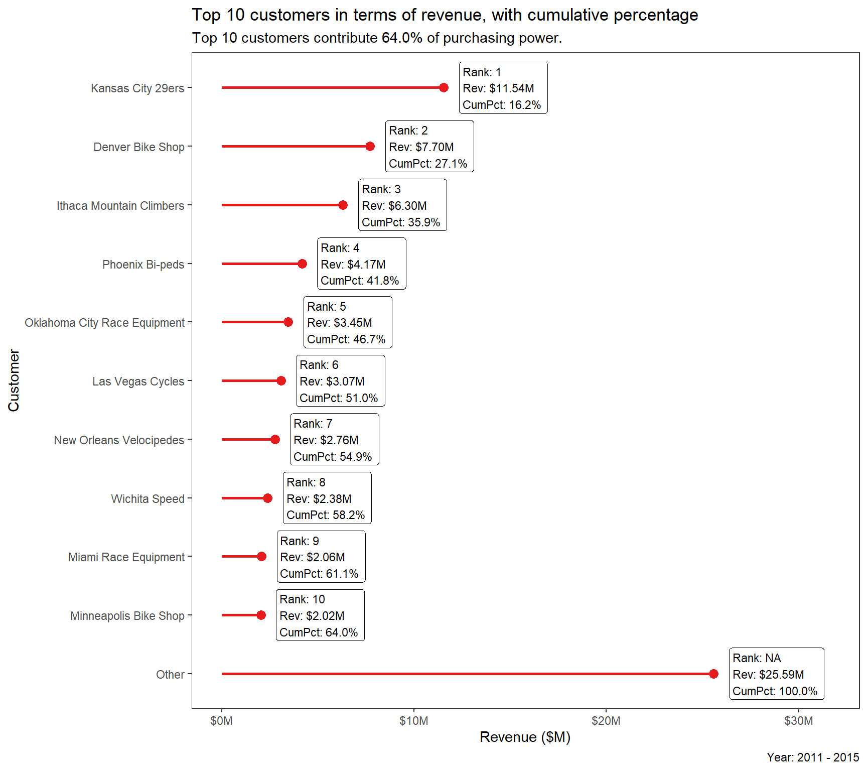
Heatmap: Customers’ Purchasing Habits
Question: Do specific customers have a purchasing preference?
Goal is to visualize heatmap of proportion of sales by Secondary Product Category.
Data manipulation
pct_sales_by_customer <- bike_orderlines %>%
  select(bikeshop_name, category_1, category_2, quantity) %>%
  group_by(bikeshop_name, category_1, category_2) %>%
  summarise(total_qty = sum(quantity)) %>%
  ungroup() %>%
  group_by(bikeshop_name) %>%
  mutate(pct = total_qty / sum(total_qty)) %>%
  ungroup() %>%
  mutate(bikeshop_name = as.factor(bikeshop_name) %>% fct_rev()) %>%
  mutate(bikeshop_name_num = as.numeric(bikeshop_name))

pct_sales_by_customer
# A tibble: 270 × 6
bikeshop_name category_1 category_2 total_qty pct bikeshop_…¹
<fct> <chr> <chr> <dbl> <dbl> <dbl>
1 Albuquerque Cycles Mountain Cross Country Race 48 0.168 30
2 Albuquerque Cycles Mountain Fat Bike 9 0.0315 30
3 Albuquerque Cycles Mountain Over Mountain 13 0.0455 30
4 Albuquerque Cycles Mountain Sport 35 0.122 30
5 Albuquerque Cycles Mountain Trail 38 0.133 30
6 Albuquerque Cycles Road Cyclocross 7 0.0245 30
7 Albuquerque Cycles Road Elite Road 69 0.241 30
8 Albuquerque Cycles Road Endurance Road 54 0.189 30
9 Albuquerque Cycles Road Triathalon 13 0.0455 30
10 Ann Arbor Speed Mountain Cross Country Race 32 0.0532 29
# … with 260 more rows, and abbreviated variable name ¹bikeshop_name_numData visualization
pct_sales_by_customer %>%
  ggplot(aes(category_2, bikeshop_name)) +
  # geometries
  geom_tile(aes(fill = pct)) +
  geom_text(aes(label = scales::percent(pct, accuracy = 0.1)),
            size = 3,
            color = ifelse(pct_sales_by_customer$pct >= 0.15, "white", "black")) +
  facet_wrap(~ category_1, scales = "free_x") +
  # formatting
  scale_fill_gradient(low = "white", high = tidyquant::palette_light()[1]) +
  labs(title = "Heatmap of Purchasing Habits",
       subtitle = str_glue("Year: {year(min(bike_orderlines$order_date))} - {year(max(bike_orderlines$order_date))}"),
       x = "Bike Type",
       y = "Customer") +
  # theme
  theme(legend.position = "none",
        axis.text.x = element_text(angle = 45, hjust = 1),
        plot.title = element_text(face = "bold"),
        strip.background = element_rect(fill = tidyquant::palette_light()[1],
                                        color = "white"),
        strip.text = element_text(color = "white", size = 11),
        panel.background = element_rect(fill = "white"))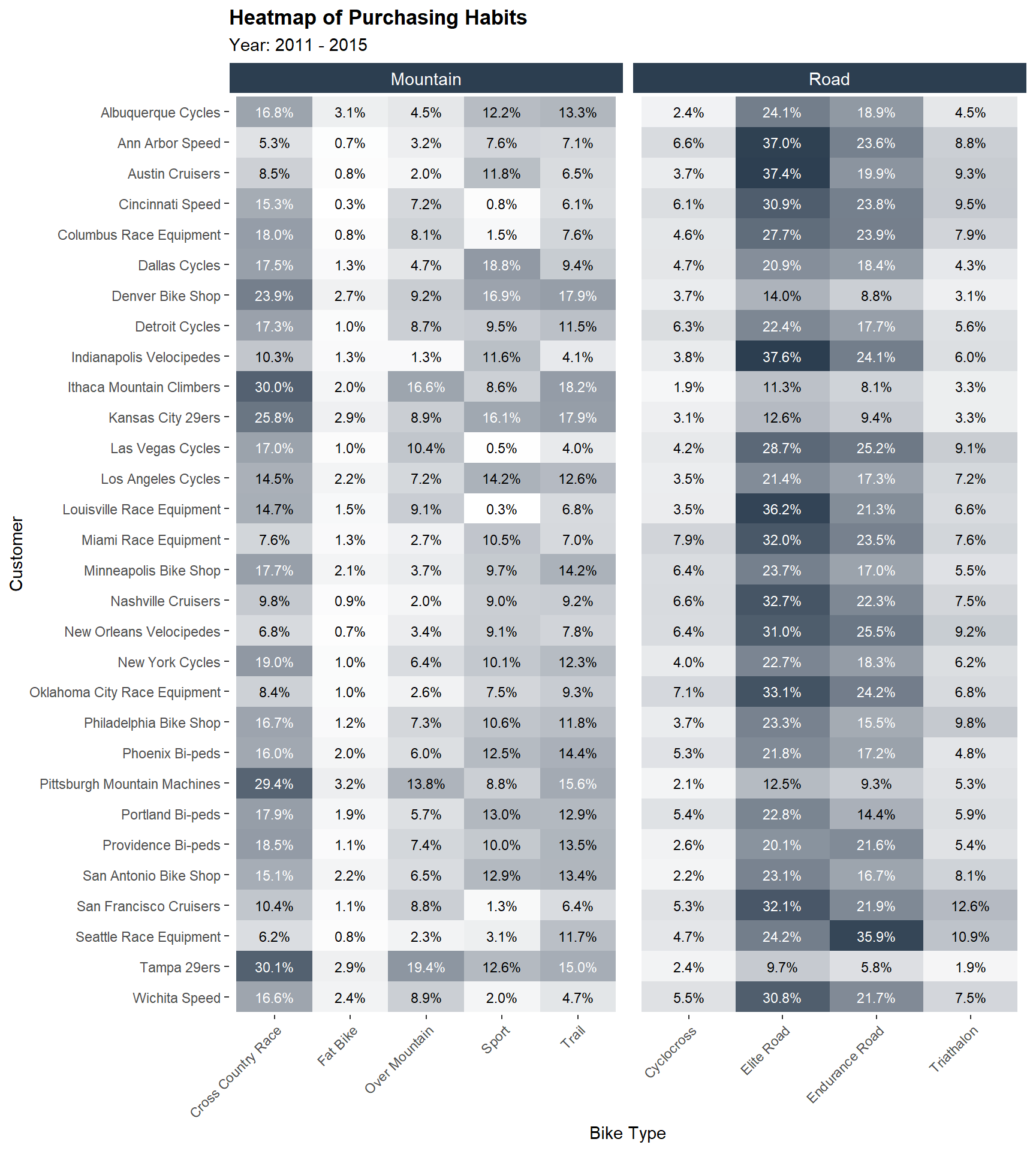
Top 3 customers that prefer mountain bikes:
- Ithaca Mountain Climbers
- Pittsburgh Mountain Machines
- Tampa 29ers
Top 3 customers that prefer road bikes:
- Ann Arbor Speed
- Austin Cruisers
- Indianapolis Velocipedes
That’s it! I hope you like it. For those wondering where I learned to make plots like this… in a fabulous course Data Science for Business Part 1 by Matt Dancho. This is probably the best course on R and I highly recommend it.