
Introduction
The aim of this project is to explore a modified version of the Chinook database using SQL and answer some business questions. The Chinook database represents a fictional digital media shop, based on real data from an iTunes Library and manually generated data. The database is provided as a SQLite database file called chinook.db.
Here’s a schema diagram for the Chinook database:
Connecting to the Database and Data Overview
library(DBI)

db <- dbConnect(RSQLite::SQLite(), dbname = "data/chinook.db")
Listing all tables in the Chinook database.
SELECT
  name,
  type
FROM sqlite_master
WHERE type IN ("table", "view")| name | type |
|---|---|
| album | table |
| artist | table |
| customer | table |
| employee | table |
| genre | table |
| invoice | table |
| invoice_line | table |
| media_type | table |
| playlist | table |
| playlist_track | table |
| track | table |
The database consists of 11 tables containing information about artists, albums, media tracks, playlists, invoices, customers, and shop employees. Let’s start by getting familiar with our data from the main tables:
employee table
SELECT *
FROM employee
LIMIT 5
customer table
SELECT *
FROM customer
LIMIT 5
invoice table
SELECT *
FROM invoice
LIMIT 5
invoice_line table
SELECT *
FROM invoice_line
LIMIT 30
track table
SELECT *
FROM track
LIMIT 20
1. Selecting Albums to Purchase
The Chinook record store has just signed a deal with a new record label, and you’ve been tasked with selecting the first three albums that will be added to the store, from a list of four. All four albums are by artists that don’t have any tracks in the store right now - we have the artist names, and the genre of music they produce:
| Artist Name | Genre |
|---|---|
| Regal | Hip-Hop |
| Red Tone | Punk |
| Meteor and the Girls | Pop |
| Slim Jim Bites | Blues |
The record label specializes in artists from the USA, and they have given Chinook some money to advertise the new albums in the USA, so we’re interested in finding out which genres sell the best in the USA.
You’ll need to write a query to find out which genres sell the most tracks in the USA, write up a summary of your findings, and make a recommendation for the three artists whose albums we should purchase for the store.
Instructions
Write a query that returns each genre, with the number of tracks sold in the USA:
- in absolute numbers
- in percentages.
Write a paragraph that interprets the data and makes a recommendation for the three artists whose albums we should purchase for the store, based on sales of tracks from their genres.
SELECT
  g.name AS genre,
  SUM(il.quantity) AS tracks_sold,
  ROUND(CAST(SUM(il.quantity) AS FLOAT)/
  (
    SELECT SUM(il.quantity)
    FROM invoice i
    INNER JOIN invoice_line il
    ON i.invoice_id = il.invoice_id
    WHERE i.billing_country = 'USA'
  )
  , 4) AS percentage_sold
FROM invoice i
INNER JOIN invoice_line il
ON i.invoice_id = il.invoice_id
INNER JOIN track t
ON il.track_id = t.track_id
INNER JOIN genre g
ON t.genre_id = g.genre_id
WHERE i.billing_country = 'USA'
GROUP BY genre
ORDER BY tracks_sold DESC| genre | tracks_sold | percentage_sold |
|---|---|---|
| Rock | 561 | 0.5338 |
| Alternative & Punk | 130 | 0.1237 |
| Metal | 124 | 0.1180 |
| R&B/Soul | 53 | 0.0504 |
| Blues | 36 | 0.0343 |
| Alternative | 35 | 0.0333 |
| Pop | 22 | 0.0209 |
| Latin | 22 | 0.0209 |
| Hip Hop/Rap | 20 | 0.0190 |
| Jazz | 14 | 0.0133 |
| Easy Listening | 13 | 0.0124 |
| Reggae | 6 | 0.0057 |
| Electronica/Dance | 5 | 0.0048 |
| Classical | 4 | 0.0038 |
| Heavy Metal | 3 | 0.0029 |
| Soundtrack | 2 | 0.0019 |
| TV Shows | 1 | 0.0010 |
Code
library(tidyverse)
theme_set(theme_classic())

genre_of_interest <- c("Alternative & Punk", "Hip Hop/Rap", "Pop", "Blues")

genre_perc %>%
  mutate(of_interest = ifelse(genre %in% genre_of_interest, "yes", "no"),
         perc_text = scales::percent(percentage_sold, accuracy = 0.1)) %>%
  ggplot(aes(x=tracks_sold, y=reorder(genre, tracks_sold, sum), fill=of_interest)) +
  geom_bar(stat = 'identity', width = 0.7) +
  geom_text(aes(label = perc_text), hjust = -0.2) +
  labs(title = "Sold Tracks by Genre, USA", x = "Tracks Sold", y = "Genre",
       fill = "Genre of Interest") +
  scale_fill_manual(values = c("gray74", "orange")) +
  scale_x_continuous(limits = c(0, 600)) +
  theme(legend.position = "top")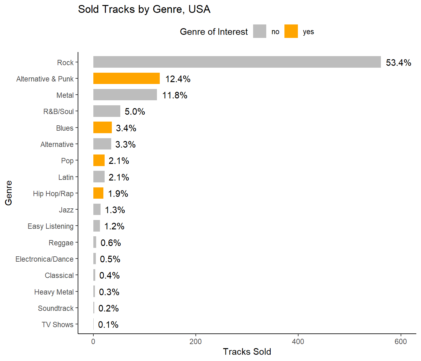
The most popular genres in the USA are Rock, Alternative & Punk, and Metal, followed with a big gap by all the others. Since our choice is limited by Hip-Hop, Punk, Pop, and Blues genres, and since we have to choose 3 out of 4 albums, we should purchase the new albums by the following artists:
- Red Tone (Punk)
- Slim Jim Bites (Blues)
- Meteor and the Girls (Pop)
2. Analyzing Employee Sales Performance
Each customer for the Chinook store gets assigned to a sales support agent within the company when they first make a purchase. You have been asked to analyze the purchases of customers belonging to each employee to see if any sales support agent is performing either better or worse than the others.
You might like to consider whether any extra columns from the employee table explain any variance you see, or whether the variance might instead be indicative of employee performance.
Instructions
Write a query that finds the total dollar amount of sales assigned to each sales support agent within the company. Add any extra attributes for that employee that you find are relevant to the analysis.
Write a short statement describing your results, and providing a possible interpretation.
SELECT
  e.first_name || ' ' || e.last_name AS sales_support_agent,
  e.hire_date,
  COUNT(DISTINCT c.customer_id) AS customers,
  SUM(i.total) AS total_sales
FROM employee e
INNER JOIN customer c
ON e.employee_id = c.support_rep_id
INNER JOIN invoice i
ON c.customer_id = i.customer_id
GROUP BY sales_support_agent| sales_support_agent | hire_date | customers | total_sales |
|---|---|---|---|
| Jane Peacock | 2017-04-01 00:00:00 | 21 | 1731.51 |
| Margaret Park | 2017-05-03 00:00:00 | 20 | 1584.00 |
| Steve Johnson | 2017-10-17 00:00:00 | 18 | 1393.92 |
While there is a 20% difference in sales between Jane (the top employee) and Steve (the bottom employee), the difference roughly corresponds with the differences in their hiring dates.
3. Analyzing Sales by Country
Your next task is to analyze the sales data for customers from each different country. You have been given guidance to use the country value from the customers table, and ignore the country from the billing address in the invoice table.
Instructions
Write a query that collates data on purchases from different countries.
Where a country has only one customer, collect them into an “Other” group.
The results should be sorted by the total sales from highest to lowest, with the “Other” group at the very bottom.
For each country, include:
- total number of customers
- total value of sales
- average value of sales per customer
- average order value
WITH t1 AS (
  SELECT
    CASE
      WHEN COUNT(DISTINCT c.customer_id) = 1 THEN 'Other'
      ELSE c.country
      END AS country,
    COUNT(DISTINCT c.customer_id) AS customers,
    SUM(i.total) AS total_sales,
    SUM(i.total)/COUNT(DISTINCT c.customer_id) AS avg_sales_per_cust,
    AVG(i.total) AS avg_order
  FROM customer c
  INNER JOIN invoice i
  ON c.customer_id = i.customer_id
  GROUP BY country
)

SELECT
  country,
  SUM(customers) AS customers,
  SUM(total_sales) AS total_sales,
  AVG(avg_sales_per_cust) AS avg_sales_per_cust,
  AVG(avg_order) AS avg_order
FROM
  (
    SELECT
      t1.*,
      CASE
        WHEN country = 'Other' THEN 1
        ELSE 0
        END AS sorted
    FROM t1
  )
GROUP BY country
ORDER BY sorted, total_sales DESC| country | customers | total_sales | avg_sales_per_cust | avg_order |
|---|---|---|---|---|
| USA | 13 | 1040.49 | 80.03769 | 7.942672 |
| Canada | 8 | 535.59 | 66.94875 | 7.047237 |
| Brazil | 5 | 427.68 | 85.53600 | 7.011147 |
| France | 5 | 389.07 | 77.81400 | 7.781400 |
| Germany | 4 | 334.62 | 83.65500 | 8.161463 |
| Czech Republic | 2 | 273.24 | 136.62000 | 9.108000 |
| United Kingdom | 3 | 245.52 | 81.84000 | 8.768571 |
| Portugal | 2 | 185.13 | 92.56500 | 6.383793 |
| India | 2 | 183.15 | 91.57500 | 8.721429 |
| Other | 15 | 1094.94 | 72.99600 | 7.445071 |
Code
sales_by_country %>%
  select(country, customers, total_sales) %>%
  mutate(country = factor(country, levels = c(country)) %>% fct_rev()) %>%
  mutate(customers = customers/sum(customers),
         total_sales = total_sales/sum(total_sales)) %>%
  pivot_longer(-country, names_to = "variable", values_to = "value") %>%
  ggplot(aes(x=value, y=country, fill=variable)) +
  geom_bar(stat = "identity", width = 0.65, position = position_dodge(0.8)) +
  labs(title="Share of Customers and Sales by Country", x="share", fill="") +
  scale_x_continuous(labels = scales::percent) +
  scale_fill_manual(values = c("gray77", "seagreen3")) +
  theme(legend.position = "top")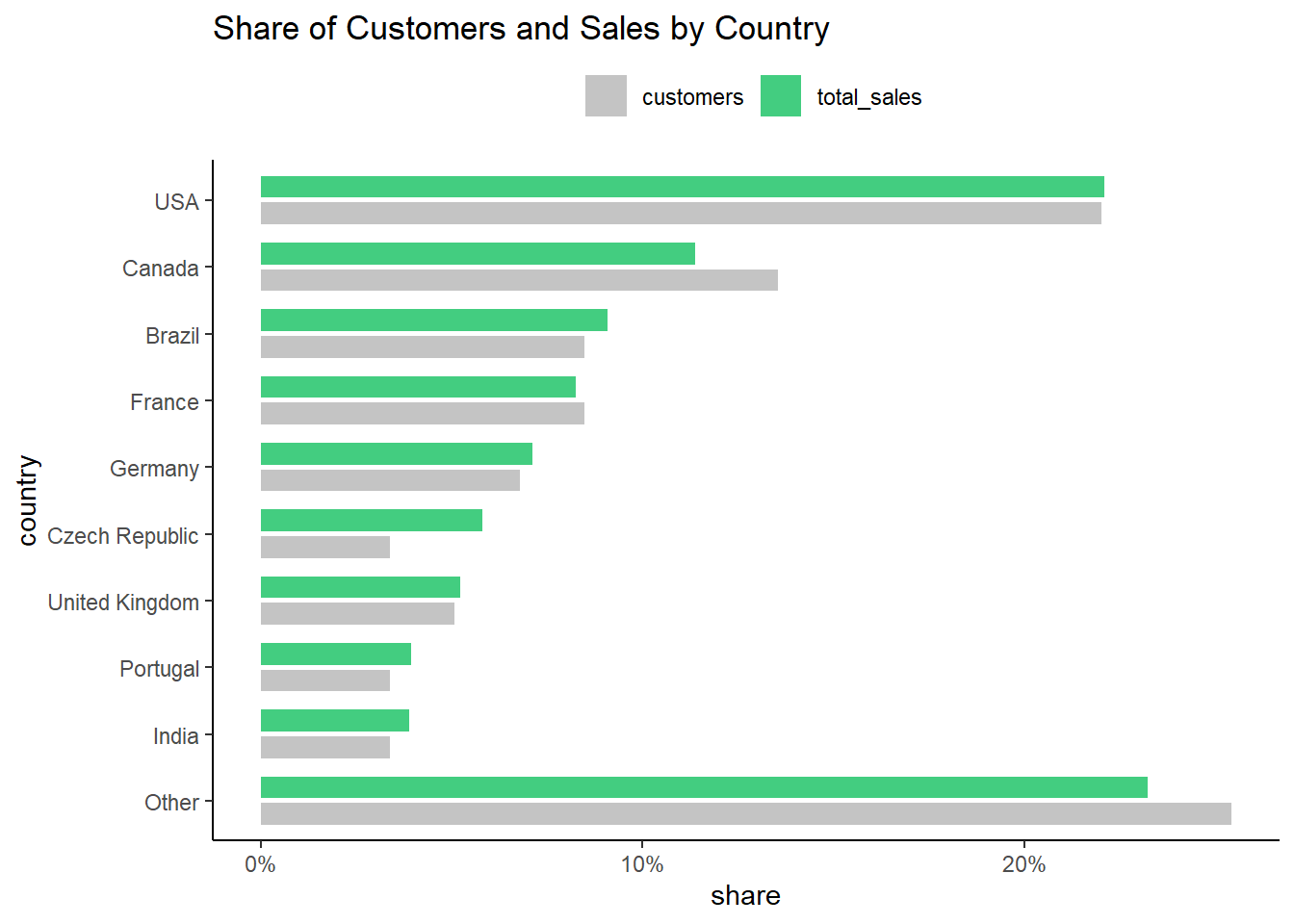
Code
sales_by_country %>%
  select(country, avg_order, avg_sales_per_cust) %>%
  mutate(country = factor(country, levels = c(country)) %>% fct_rev()) %>%
  mutate(avg_order = (avg_order - mean(avg_order)) / mean(avg_order),
         avg_sales_per_cust = (avg_sales_per_cust - mean(avg_sales_per_cust)) /
                                 mean(avg_sales_per_cust)) %>%
  rename(`Average Order` = avg_order,
         `Average Sales per Customer` = avg_sales_per_cust) %>%
  pivot_longer(-country, names_to = "variable", values_to = "pct_diff_from_mean") %>%
  ggplot(aes(x=pct_diff_from_mean, y=country, fill=variable)) +
  geom_col(width = 0.65, position = position_dodge(0.8)) +
  facet_wrap(~ variable, scales = "free_x") +
  labs(title="Average Order & Average Sales per Customer",
       subtitle = "(Percent Difference from Mean)", x="pct diff from mean", fill="") +
  scale_fill_manual(values = c("steelblue", "lightskyblue2")) +
  scale_x_continuous(labels = scales::percent) +
  theme(legend.position = "top")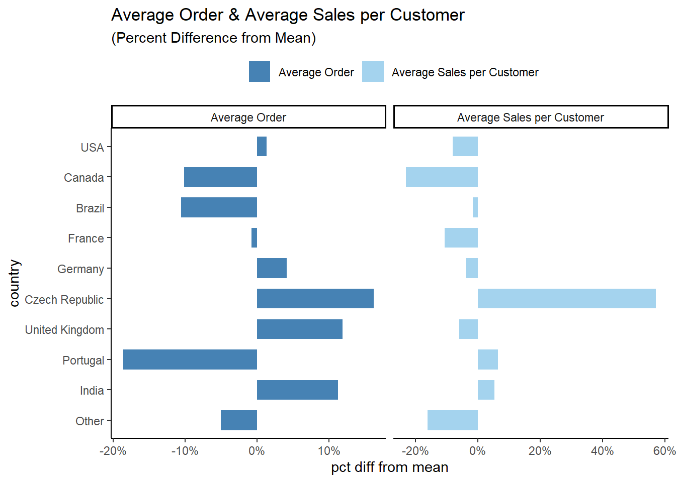
The USA has the largest customer base and, consequently, the highest total sales.
Based on the data, there may be opportunity in the following countries:
- Czech Republic
- United Kingdom
- India
It’s worth keeping in mind that the amount of data from each of these countries is relatively low. Because of this, we should be cautious spending too much money on new marketing campaigns, as the sample size is not large enough to give us high confidence. A better approach would be to run small campaigns in these countries, collecting and analyzing the new customers to make sure that these trends hold with new customers.
4. Albums vs Individual Tracks
The Chinook store is setup in a way that allows customer to make purchases in one of the two ways:
- purchase a whole album
- purchase a collection of one or more individual tracks.
The store does not let customers purchase a whole album, and then add individual tracks to that same purchase (unless they do that by choosing each track manually). When customers purchase albums they are charged the same price as if they had purchased each of those tracks separately.
Management are currently considering changing their purchasing strategy to save money. The strategy they are considering is to purchase only the most popular tracks from each album from record companies, instead of purchasing every track from an album.
We have been asked to find out what percentage of purchases are individual tracks vs whole albums, so that management can use this data to understand the effect this decision might have on overall revenue.
Instructions
Write a query that categorizes each invoice as either an album purchase or not, and calculates the following summary statistics:
- Number of invoices
- Percentage of invoices
Write one to two sentences explaining your findings, and making a prospective recommendation on whether the Chinook store should continue to buy full albums from record companies
WITH cat_purchase AS (
  SELECT
    il.invoice_id,
    CASE
      WHEN
      COUNT(DISTINCT t.album_id) = 1
      AND
      COUNT(DISTINCT t.track_id) = c.count_album_tracks
      THEN 'album'
      ELSE 'individual track(s)'
      END AS purchase_type,
      c.count_album_tracks
    FROM track t
    JOIN invoice_line il
    ON il.track_id = t.track_id
    JOIN (SELECT COUNT(*) AS count_album_tracks, album_id
          FROM track
          GROUP BY album_id) c
    ON c.album_id = t.album_id
    GROUP BY invoice_id
)

SELECT
  purchase_type,
  COUNT(*) AS number_of_invoices,
  ROUND(CAST(COUNT(*) AS float) / CAST(
    (SELECT COUNT(*)
    FROM invoice) AS FLOAT), 2) AS percentage_of_invoices
FROM cat_purchase
GROUP BY purchase_type| purchase_type | number_of_invoices | percentage_of_invoices |
|---|---|---|
| album | 114 | 0.19 |
| individual track(s) | 500 | 0.81 |
Album purchases account for 19% of all purchases. Based on this data, I would recommend against purchasing only the most popular tracks from each album from record companies, since there is a potential of losing a significant portion of revenue.
5. Which artist is used in the most playlists?
SELECT
  ar.name AS artist,
  g.name AS genre,
  COUNT(DISTINCT pt.playlist_id) AS number_of_playlists,
  COUNT(DISTINCT t.track_id) AS unique_tracks
FROM artist ar
JOIN album al ON ar.artist_id=al.artist_id
JOIN track t ON al.album_id=t.album_id
JOIN playlist_track pt ON pt.track_id = t.track_id
JOIN genre g ON g.genre_id = t.genre_id
GROUP BY artist, genre
ORDER BY number_of_playlists DESC, unique_tracks DESC| artist | genre | number_of_playlists | unique_tracks |
|---|---|---|---|
| Eugene Ormandy | Classical | 7 | 3 |
| Berliner Philharmoniker & Herbert Von Karajan | Classical | 6 | 3 |
| The King’s Singers | Classical | 6 | 2 |
| English Concert & Trevor Pinnock | Classical | 6 | 2 |
| Academy of St. Martin in the Fields & Sir Neville Marriner | Classical | 6 | 2 |
| Michael Tilson Thomas & San Francisco Symphony | Classical | 5 | 2 |
| Yo-Yo Ma | Classical | 5 | 1 |
| Wilhelm Kempff | Classical | 5 | 1 |
| Ton Koopman | Classical | 5 | 1 |
| Sir Georg Solti, Sumi Jo & Wiener Philharmoniker | Opera | 5 | 1 |
Eugene Ormandy takes the first place with only 3 unique tracks in 7 different playlists. His music belongs to the classical genre, which we have previously seen is one of the least popular genres in the USA.
If we order this table by number of unique tracks, we get a completely different list.
SELECT
  ar.name AS artist,
  g.name AS genre,
  COUNT(DISTINCT pt.playlist_id) AS number_of_playlists,
  COUNT(DISTINCT t.track_id) AS unique_tracks
FROM artist ar
JOIN album al ON ar.artist_id=al.artist_id
JOIN track t ON al.album_id=t.album_id
JOIN playlist_track pt ON pt.track_id = t.track_id
JOIN genre g ON g.genre_id = t.genre_id
GROUP BY artist, genre
ORDER BY unique_tracks DESC, number_of_playlists DESC| artist | genre | number_of_playlists | unique_tracks |
|---|---|---|---|
| Led Zeppelin | Rock | 3 | 114 |
| Metallica | Metal | 4 | 112 |
| U2 | Rock | 3 | 112 |
| Iron Maiden | Metal | 4 | 95 |
| Deep Purple | Rock | 3 | 92 |
| Iron Maiden | Rock | 3 | 81 |
| Pearl Jam | Rock | 4 | 54 |
| Van Halen | Rock | 3 | 52 |
| Os Paralamas Do Sucesso | Latin | 3 | 49 |
| Lost | TV Shows | 2 | 48 |
6. How many tracks have been purchased vs not purchased?
WITH all_and_purchased_tracks AS (
  SELECT
    t.track_id AS all_tracks,
    il.track_id AS purch_tracks
  FROM track t
  LEFT JOIN invoice_line il
  ON t.track_id = il.track_id
)

SELECT
  COUNT(DISTINCT all_tracks) AS total_tracks,
  COUNT(DISTINCT purch_tracks) AS pirchased,
  COUNT(DISTINCT all_tracks) - COUNT(DISTINCT purch_tracks) AS not_purchased,
  ROUND(CAST(COUNT(DISTINCT purch_tracks) AS FLOAT)/COUNT(DISTINCT all_tracks), 3)
    AS perc_purchased,
  ROUND(CAST(COUNT(DISTINCT all_tracks) - COUNT(DISTINCT purch_tracks)
    AS FLOAT)/COUNT(DISTINCT all_tracks), 3)
    AS perc_not_purchased
FROM all_and_purchased_tracks| total_tracks | pirchased | not_purchased | perc_purchased | perc_not_purchased |
|---|---|---|---|---|
| 3503 | 1806 | 1697 | 0.516 | 0.484 |
Code
pie(c(51.6, 48.4), labels = c("purchased", "not purchased"),
    main = "Purchased vs not purchased tracks")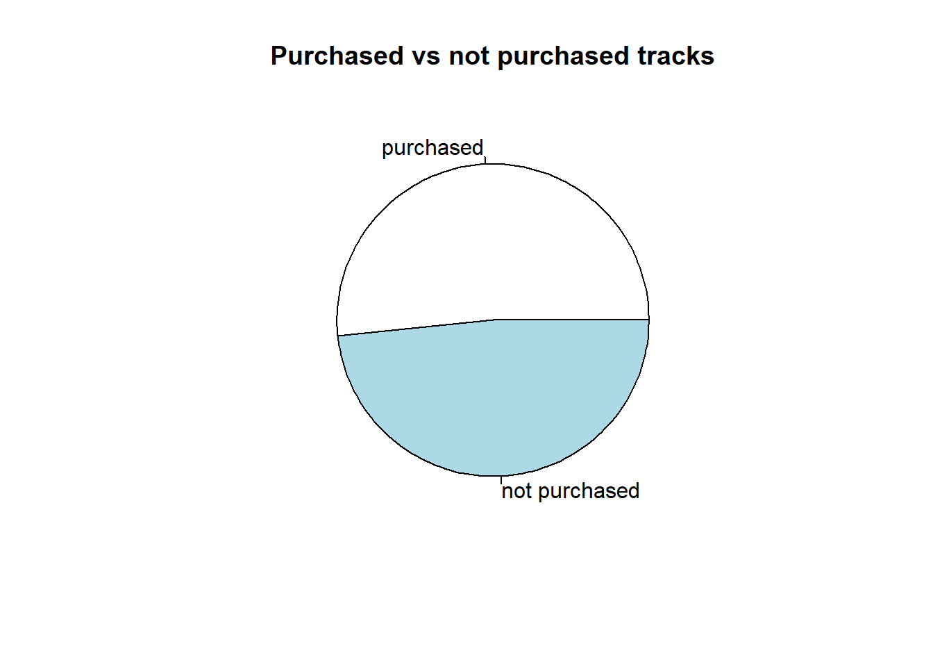
Almost half of all the unique tracks available in the Chinook store were never bought, probably being of unpopular genre or unpopular artists.
7. Do protected vs non-protected media types have an effect on popularity?
Let’s take a look at the media_type table.
SELECT *
FROM media_type| media_type_id | name |
|---|---|
| 1 | MPEG audio file |
| 2 | Protected AAC audio file |
| 3 | Protected MPEG-4 video file |
| 4 | Purchased AAC audio file |
| 5 | AAC audio file |
There are 2 out of 5 media types that are protected.
WITH t AS (
  SELECT
    t.track_id,
    CASE
      WHEN mt.name LIKE "%protected%" THEN "yes" ELSE "no"
      END AS protected
  FROM track t
  JOIN media_type mt ON mt.media_type_id = t.media_type_id
)

SELECT
  protected,
  COUNT(DISTINCT t.track_id) AS unique_tracks,
  ROUND(CAST(COUNT(DISTINCT t.track_id) AS FLOAT) / (SELECT COUNT(*) FROM track), 2)
    AS 'unique_tracks_%',
  COUNT(DISTINCT il.track_id) AS sold_unique_tracks,
  COUNT(il.track_id) AS sold_tracks,
  ROUND(CAST(COUNT(il.track_id) AS FLOAT) / (SELECT COUNT(*) FROM invoice_line), 2)
    AS 'sold_tracks_%'
FROM t
LEFT JOIN invoice_line il ON t.track_id = il.track_id
GROUP BY protected| protected | unique_tracks | unique_tracks_% | sold_unique_tracks | sold_tracks | sold_tracks_% |
|---|---|---|---|---|---|
| no | 3052 | 0.87 | 1652 | 4315 | 0.91 |
| yes | 451 | 0.13 | 154 | 442 | 0.09 |
Code
by_media_type %>%
  select(protected, unique_tracks, sold_tracks) %>%
  rename(unique = unique_tracks,
         sold = sold_tracks) %>%
  pivot_longer(-protected, names_to = "tracks", values_to = "count") %>%
  mutate(tracks = as.factor(tracks) %>% fct_rev()) %>%
  group_by(tracks) %>%
  mutate(pct = count/sum(count) %>% round(2)) %>%
  ungroup() %>%
  ggplot(aes(x=tracks, y=count, fill=protected)) +
  geom_col(width = 0.5, position = "stack", color = "white") +
  geom_text(aes(label = count), position = position_stack(vjust = .5),
            color = "white", fontface = "bold")+
  scale_fill_manual(values = c("#fbc02d", "#03a9f4")) +
  theme(legend.position = "top")
by_media_type %>%
  select(protected, unique_tracks, sold_unique_tracks) %>%
  rename(unique = unique_tracks,
         unique_sold = sold_unique_tracks) %>%
  mutate(unique_unsold = unique - unique_sold) %>%
  pivot_longer(-protected, names_to = "tracks", values_to = "count") %>%
  filter(tracks != "unique") %>%
  group_by(protected) %>%
  mutate(percentage = scales::percent(count/sum(count), accuracy = 0.1)) %>%
  ggplot(aes(x=protected, y=count, fill=tracks)) +
  geom_col(width = 0.5, position = "fill", color = "white") +
  scale_fill_manual(values = c("seagreen3", "tomato")) +
  geom_text(aes(label = percentage), position = position_fill(vjust = .5),
            color = "white", fontface = "bold") +
  labs(y="proportion") +
  theme(legend.position = "top")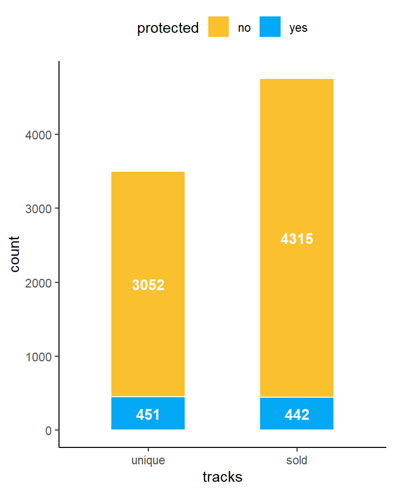
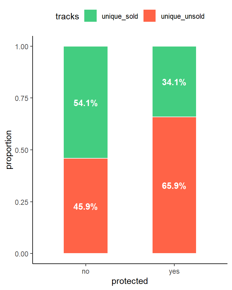
We can make the following observations:
- Only 13% of all the unique tracks available in the Chinook store are of protected media types.
- Among all the tracks that were sold, those of protected media types amounts only to 9%.
- From all the unique tracks of protected media types, only 34,1% were sold, while from those of non-protected ones 54,1%.
We can conclude that the tracks of protected media types are much less popular than those of non-protected.